Snowball Earth Theory Simulation
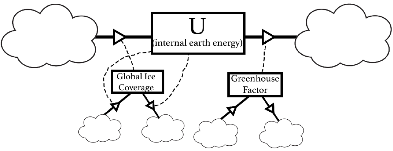
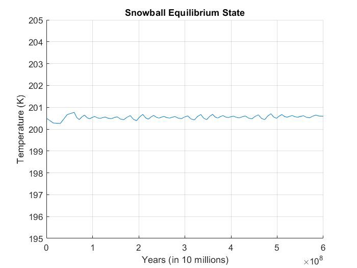
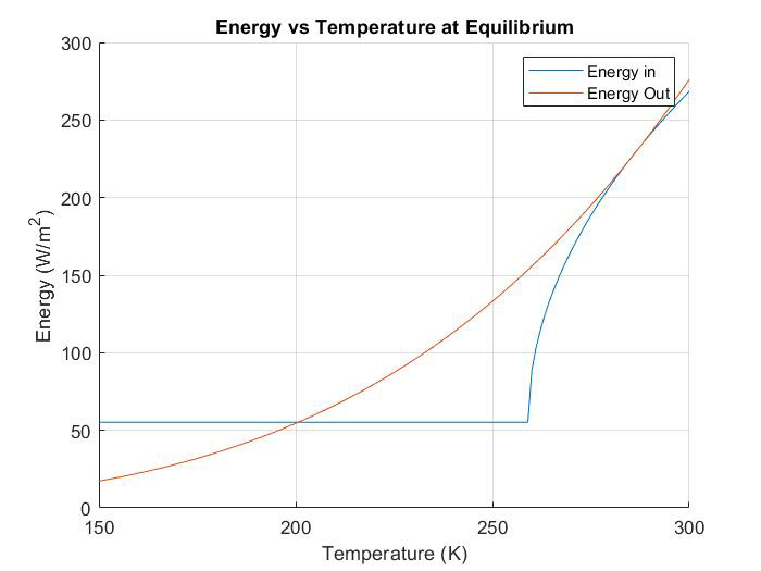
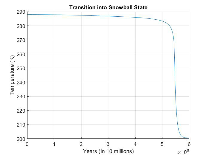
The goal of this project was to explore a possible explanation for how the Earth would transition into a snowball state. The snowball state is when the entire earth is covered in ice. It is estimated Earth has been in this state twice. The flow diagram represents how energy, ice coverage and greenhouse factor interact. The Energy vs Temperature at Equilibrium graph represent the energy in and out needed to maintain an the given equilibrium temperature, The Transition into Snowball State graph shows the temperature as CO2 level are decreased over time. For a full explanation click here for the computational essay.
Comparative Analysis of Air Source vs. Ground Source Heat Pump
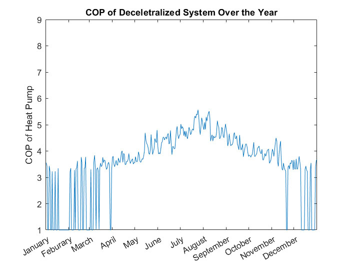
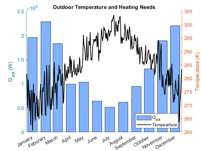
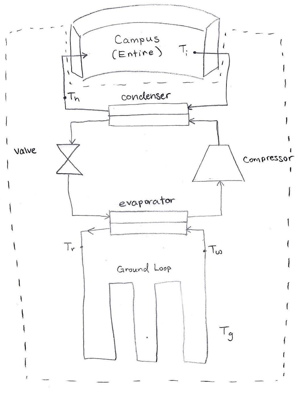
As more people switch to alternative heating methods in the New England area, a team and I developed a model to analyze the effectiveness of 2 of the most popular systems: ground-source heat pumps & air-source heat pumps. We built the model around Olin College using weather data, campus heating needs, and area ground temperatures. The simulation was developed in Matlab and analyzed several components of the system including efficiency, pump speed required, and entropy generation through advanced knowledge of thermodynamics and fluid systems with the help of REFPROP. After the model analyzed one year of performance it found that the ground-source pump was a more efficient and reliable method of heating.
Monte Carlo Localization and Bayesian Statistics
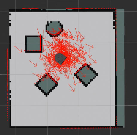
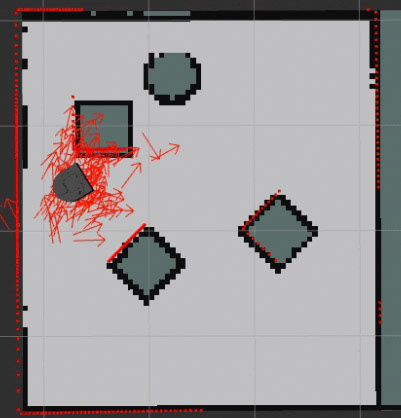
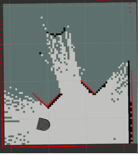
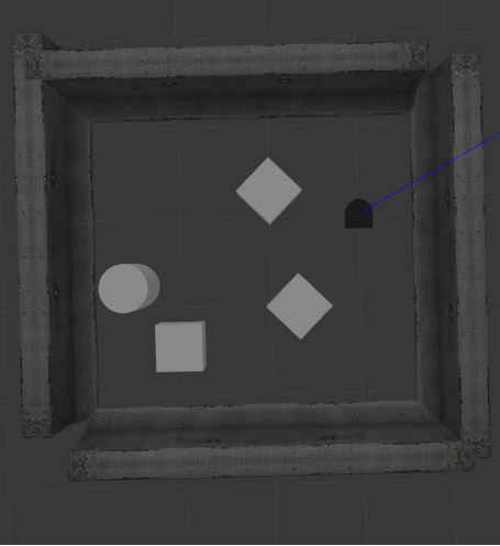
Monte Carlo Localization is rapidly becoming on of the most popular localization strategies for robotics, so given the heavy emphasize of Bayesian statistics in a Probabilistic Modeling class, my partner and I dove into the method for our final project. We chose to do this project in a virtual environment so we could better study the statics and focus less on debugging hardware. As a result we got to dive deep into understanding the connection to Bayesian statistics and conduct addition research on ways to make the program more robust. In the end, we were successfully able to accurately determine the robots locations as it drove around an area of odd shapes.
Controls Using Simulink: Inverse Pendulum
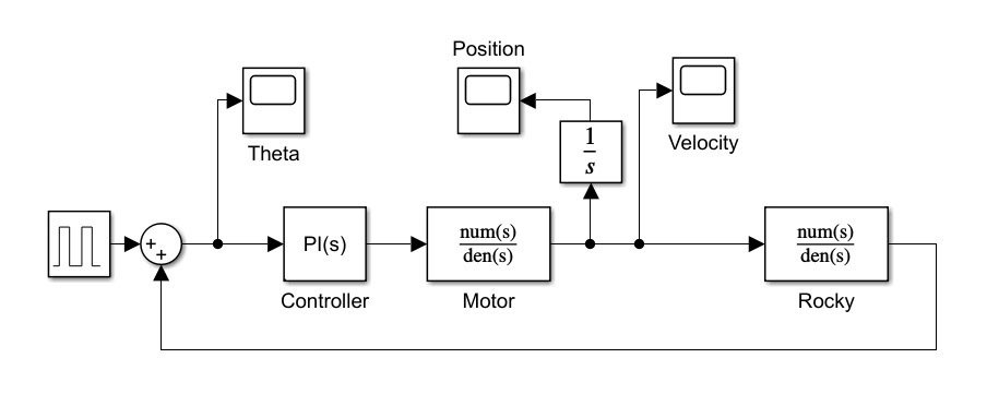
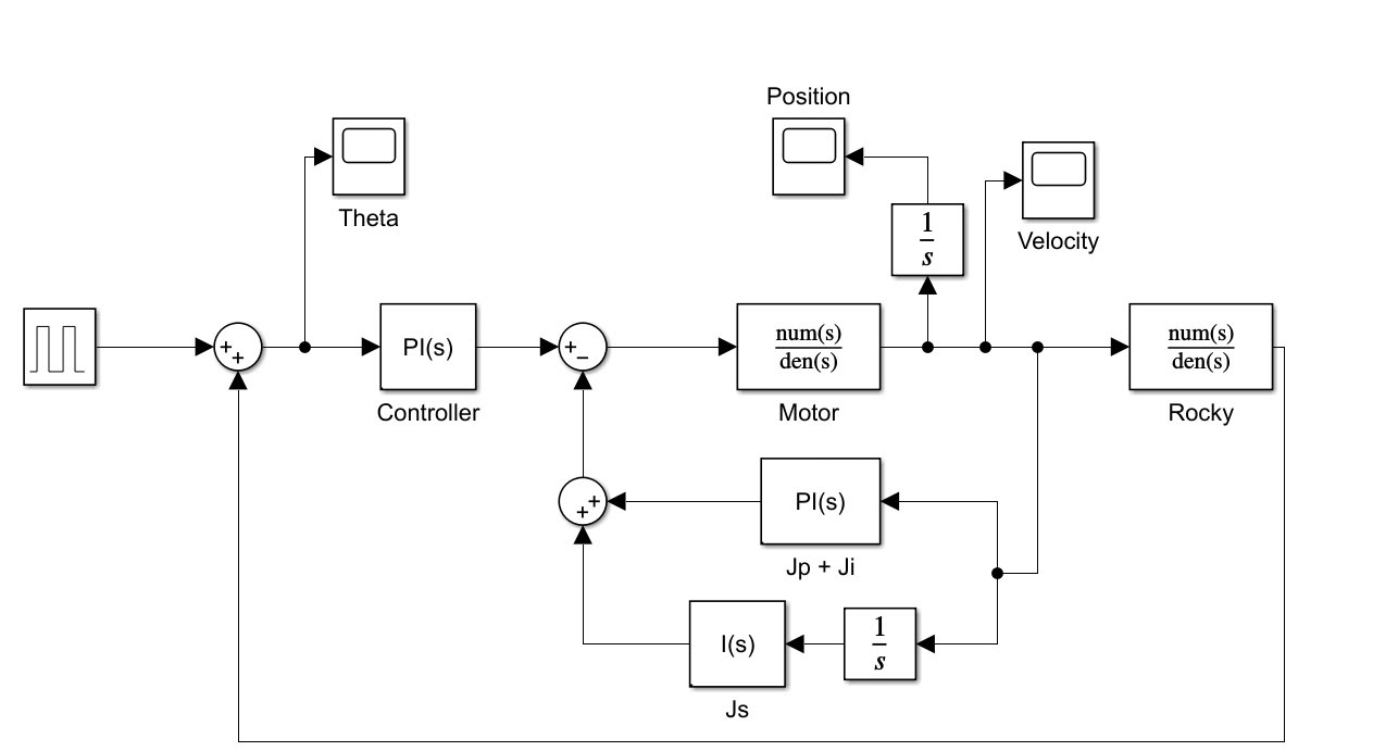
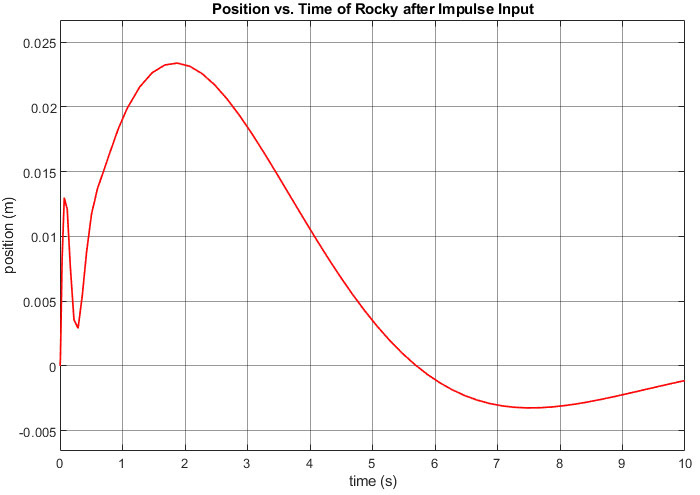
During the class Engineering Systems Anaylsis, I used laplace transforms and the MATLAB simulink program to develop and test feedback responses to an inverted pendulum.
Step Analysis using Fourier Transform
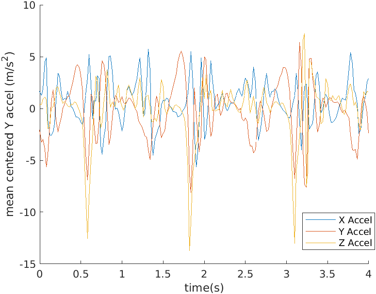
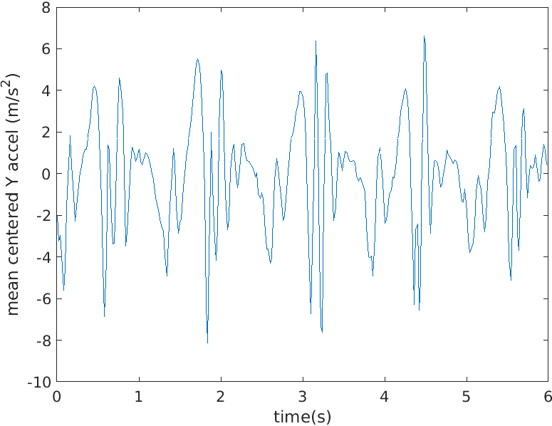
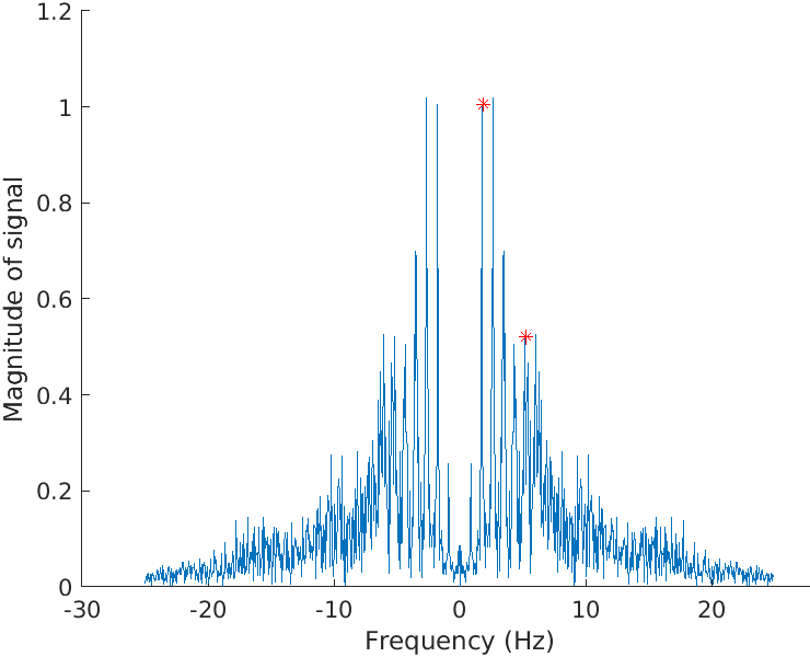
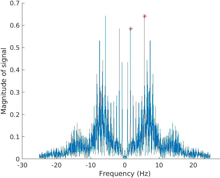
As part of a quantitative engineering analysis course, my team and I did a deep dive into utilizing the Fourier Transform and analyzing it results to draw conclusions. For this project, we specifically focused on step asymmetry as it is an important factor in determining fall risk. In order to calculate this we began by taking accelerometer data in the Y axis (vertical acceleration) from a phone in a pocket. We then took the Fourier Transform of the data to see where the highest frequencies in these occurred. The analysis of the location of these peaks allowed us to determine the quality of the step and come up with a formula to determine a score. A more in-depth analysis of the process and results can be found at the linked website.
Modeling Velocity Profile of a Train in a Tunnel
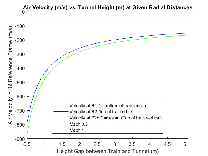
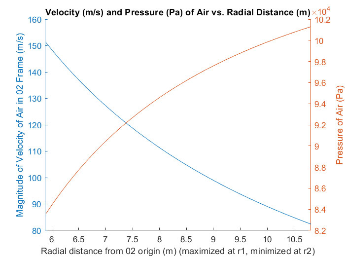
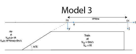
The final project of an intermediate Transport Phenomona class tasked model a real life situation using the Navier-Stokes equations. My partner and I choose to model the velocity profile of air around a train as it went through a tunnel. This required multiple mathematical approaches including shifting reference frames, convolutions, and partial derivatives. The calculation were simulated using MATLAB and a comprehensive report of the various modeling methods and processes is attach above.
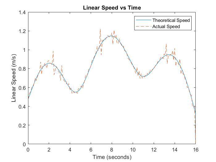
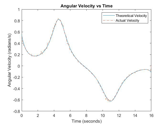
Bridge of Doom Robot Project
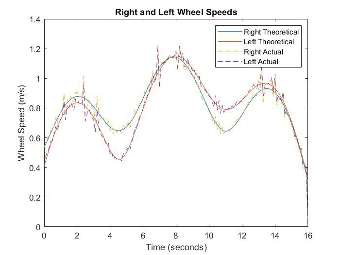
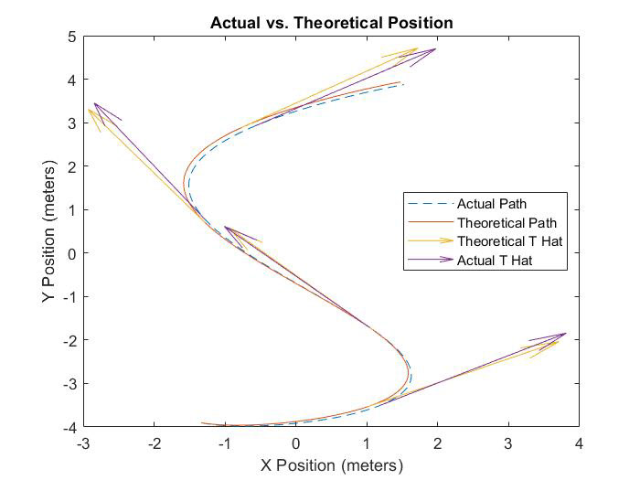
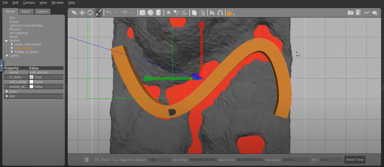
The aim of this project is to use concept of linear algebra and multivariable calculus to create a program that will allow a robot to traverse a bridge based on any given function. To code the robot we determined the linear speed and angular velocity it much travel at during each point of the bridge. From there we converted those values into wheel velocities. The values of each of the above quantities can be observed in the first three graphs to the right. After calculating the wheel speed, we then transferred our control code over to a simulation and ran the robot and got encoder data values. We used these values to calculated the actual linear speed, angular velocity, wheel speed, and position and plotted those against the ideal values as seen. For a detailed write up on how we went about calculating all of the above click here.
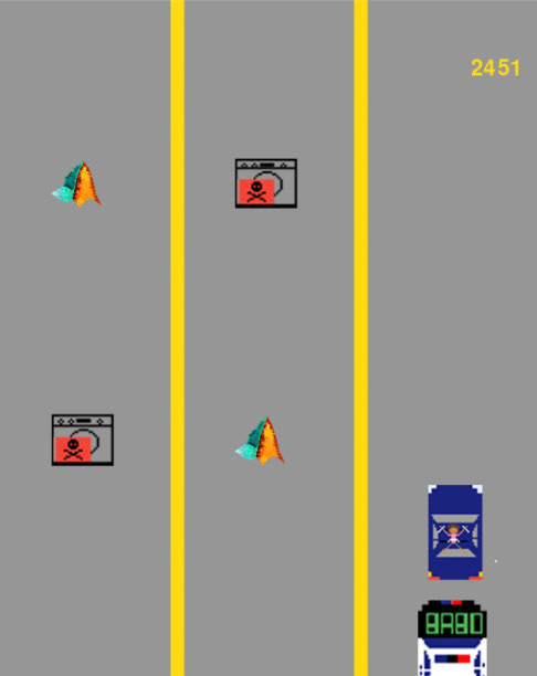
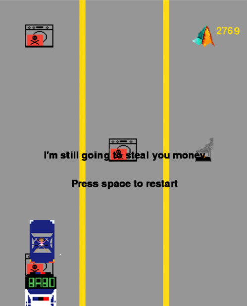
Video Game Design with Pygame
As part of a software design class, I designed a game using the Model View Controller architecture. The goal of the game was to avoid incoming obstacle while you are running away from campus police. The obstacles are all tied to school like the common broken computer, washing machine that steals money, and the powerful but frustrating matlab. The game is coded all in python and makes use of the pygame library to help in several tasks like images formatting, display, and object collisions. This project also helped with coming up with and implementing meaningful unit tests to test various aspects of the game.